Persistent Homology
Persistent homology answers one practical question:
Which holes, clusters, and voids survive as we change the distance scale?
Vietoris-Rips Complex
Given a point cloud \(X = \{x_1, \ldots, x_n\}\) and radius \(\epsilon\), the Vietoris-Rips complex is:
Plain meaning:
- if two points are within \(\epsilon\), add an edge;
- if three points are pairwise within \(\epsilon\), add a triangle;
- if four points are pairwise within \(\epsilon\), add a tetrahedron.
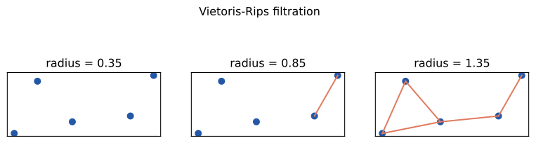
Filtration
Persistent homology does not compute one complex. It computes a sequence of complexes over increasing radius:
Each inclusion says that once an edge, triangle, or higher simplex appears, it stays available at larger radii. The useful signal is not only which topology exists, but when it appears and how long it survives.
Chains, Boundaries, And Homology
A \(k\)-simplex is a \(k\)-dimensional building block:
- 0-simplex: vertex;
- 1-simplex: edge;
- 2-simplex: triangle;
- 3-simplex: tetrahedron.
A \(k\)-chain is a formal sum of \(k\)-simplices. The boundary operator maps a simplex to its boundary:
The key algebraic fact is:
That means every boundary is already closed. Homology measures closed things that are not merely boundaries:
Plain meaning:
- \(H_0\) measures connected components;
- \(H_1\) measures loops;
- \(H_2\) measures voids.
Persistence Module
Each filtration inclusion \(K_i \subseteq K_j\) induces a map:
The sequence of homology groups and maps is a persistence module. Barcodes and persistence diagrams are compact summaries of this module.
Barcode
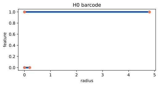
For homology dimension \(k\), the barcode is:
Each pair means one feature is born at radius \(b_i\) and dies at radius \(d_i\). Its lifetime is:
Long bars matter more because they survive more scales.
Betti Curve
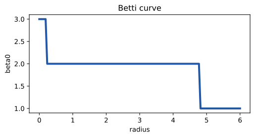
The Betti number at radius \(\epsilon\) counts live bars:
For ML, this becomes a curve feature. It says how many connected components, loops, or voids exist at each scale.
How To Read The Output
For a classifier or regressor, the diagram is not usually the final input. It is an intermediate object. Common downstream encodings include:
- Betti curves sampled at fixed radii;
- total persistence;
- persistence entropy;
- persistence images;
- persistence landscapes;
- summary statistics by dimension.
The active package currently implements diagram queries and Betti-curve feature
matrices through PHFeaturizer.
Exact Reuse Under Similarity Motion
Suppose every pairwise distance in trajectory frame \(t\) obeys
Then the Vietoris-Rips filtration is only reparameterized:
Every persistence interval transforms as
with essential deaths remaining infinite. Therefore
persistence_similarity_trajectory checks this distance condition numerically.
Its tolerance is an implementation certificate, not proof that noisy measured
motion follows an exact physical law. Anisotropic deformation, independent point
motion, and duplicate base points that later separate fail certification and use
dense recomputation. Finite filtration cutoffs also use the dense path because
the current reference reducer's cutoff changes which truncated bars appear
essential.
Failure Modes
Topology is useful when it captures structure beyond norm, density, or recency. Reject a topology feature if:
- random same-budget features perform the same;
- locality-only features perform the same;
- schedule construction costs more than it saves;
- results only work on one synthetic seed.